Subscapes (Part 3 – Code)
Technical Details
This is Part 3 of my Subscapes blog post series. In this post, I’ll break down the technical details in the rendering algorithm and explain how I made the artwork. This post assumes a general understanding of JavaScript and programming. If you haven’t already, you may want to start with Part 1 (Preface) and Part 2 (Traits).
This post is split into two topics: The Subscapes Algorithm (how it works) and Tokens as Data (some discussion around the minted tokens).
The Subscapes Algorithm
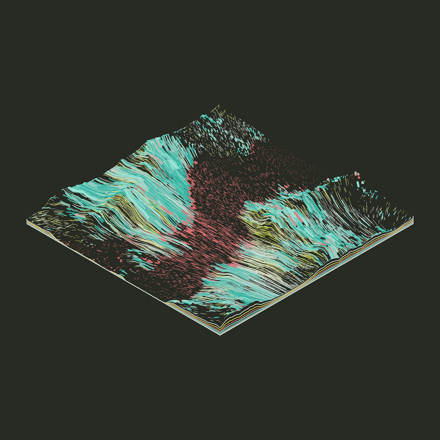
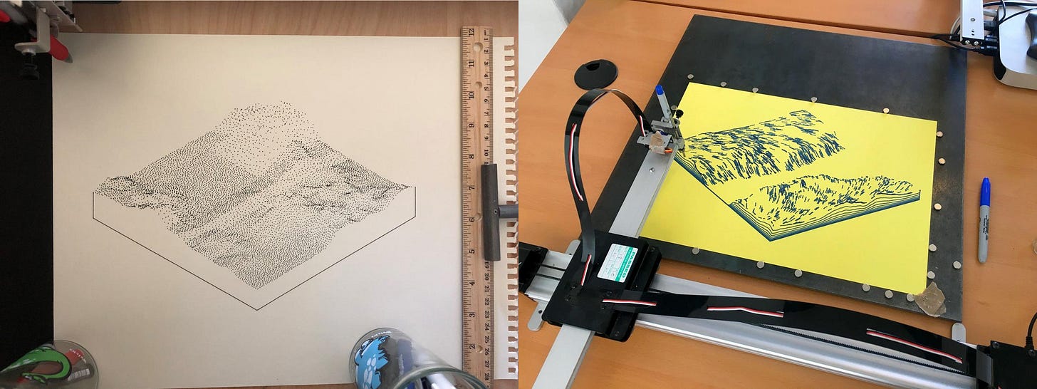
The Subscapes algorithm is a single function contained in around 17kb of minified JavaScript. When executed, the algorithm produces a series of polyline segments uniquely tied to an input hash. By default, these lines are drawn to a HTML5 <canvas> context to draw the image, but the script can also be run ‘headlessly’ to return a simple JSON structure (for example: for a mechanical plotter, CNC mill, or Node.js).
The script combines several high-level ideas in graphics programming to form the final series of images:
3D Projection — converting 3D points to 2D screen-space lines
Parametric Geometry — describing the surface with a pure function
f=(x,y)Noise — summing 2D simplex noise to determine terrain height
Quadtrees — recursive subdivision of the surface to form a quilt-like texture
Poisson Disk Sampling — distributing stroke surface positions uniformly
Flow Fields — used to create organic stroke motion across the surface
Raycasting — removing triangles that are back-facing or occluded
Diffuse Lighting — sometimes using lighting for stroke coloring
Procedural Color Selection — uniformly distributed high-contrast uniform palettes
I’ll try to break down each concept individually.
3D Projection
Something I often do in my work is convert 3D constructs into 2D primitives like lines, points, and polygons. This allows me to use a range of graphical toolkits (HTML5 Canvas, SVG, etc), but it’s also suitable for drawing with a mechanical pen plotter.
To convert 3D constructs into 2D primitives, you first need to project the coordinates from 3D world-space into 2D screen-space. To do this, I tend to use gl-matrix, which helps us construct projection matrices that we can use to transform 3D vectors.
To simplify these concepts, I tend to use virtual camera utilities, that allows me to set an eye position and target. The camera utility returns a project() function that converts 3D to 2D coordinates.
| // List of 3D coordinates | |
| const vertices = [ | |
| [-0.5, 0, -0.5], | |
| [0.5, 0, -0.5], | |
| ... | |
| ]; | |
| // A utility that projects 3D points to 2D screen-space | |
| // Using a virtual 'camera' that has a 3D position and target | |
| // And viewport width and height | |
| const position = [ 1, 1, 1 ]; | |
| const target = [ 0, 0, 0 ]; | |
| const project = createCamera({ position, target, width, height }); | |
| // Project the 3D to 2D | |
| const screenPoints = vertices.map(p => project(p)); | |
| // ... Now draw the 2D points somehow (e.g. as paths) |
I’ve created a small canvas demo showing how to achieve this kind of 3D-to-2D rendering:
Subscapes uses the same technique, but with modified code so that it is far more compact in byte size. The Subscapes camera uses an orthographic projection matrix, more specifically isometric projection, which ends up creating parallel projection lines and leads to the iconic 2.5D tiles.
Parametric Geometry
Once you have a virtual camera, you can begin to build more complex 3D structures and project them down to 2D primitives. In Subscapes, the geometry is entirely parametric; in other words, it is defined by a single function:
| function parametricTerrain ([ u, v ]) { | |
| // Turn 0..1 to -1..1 | |
| const x = u * 2 - 1; | |
| const z = v * 2 - 1; | |
| // Find height at this 2D coordinate | |
| const y = calculateTerrainHeight(x, z); | |
| // Return the 3D surface point | |
| return [ x, y, z ]; | |
| } |
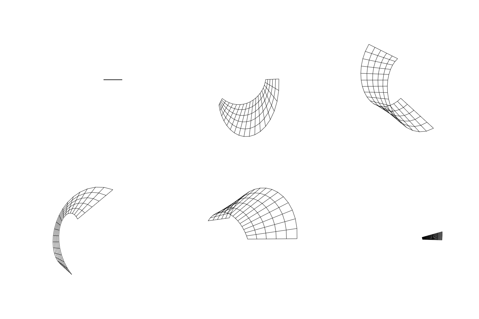
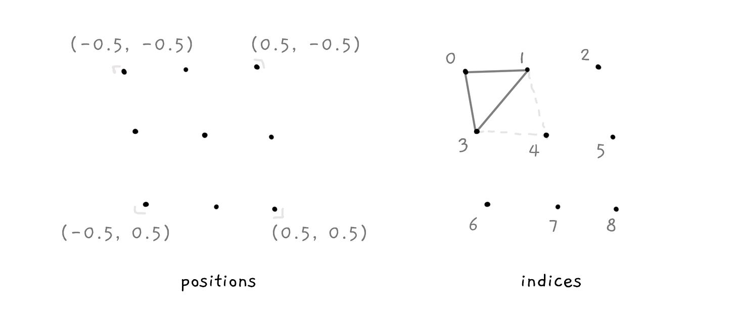
The role of the parametric function is to determine the 3D coordinate on the surface for a given (U, V) coordinate. Parametric geometries are often rendered by subdividing the surface into horizontal and vertical slices, and passing a U and V values in the range 0..1 into the function at each slice.
This gives us a list of 3D points along the geometry’s surface, and regular sets of indices that describe how to connect these vertices (e.g. as triangles or quadrilaterals).
| // Number of horizontal and vertical slices | |
| const subdivisions = 20; | |
| // Calculate vertices at each grid point and gather the triangle indices of the mesh | |
| // We pass our 'parametricTerrain' function in as an input to the generator | |
| const [ vertices, cells ] = generateGeometry(parametricTerrain, subdivisions); | |
| // vertices are 3D positions on the surface | |
| // [ [ x0, y0, z0 ], [ x1, y1, z1 ], ... ] | |
| // cells are indices into the above array, defining triangles | |
| // [ [ 0, 1, 3 ], [ 1, 4, 3 ], [ 1, 2, 4 ], ... ] |
The 3D points can then be ordered into regular sets to define the 3D triangles, quadrilaterals, or another structure.
I’ve created a small canvas demo below that shows how to use parametric 3D geometry with 2D lines. In this demo, the parametric function is a sine wave along one axis.
One of the benefits of parametric geometry is that it is very compact (no need to store a 3D model), but also that it resolution independent. To increase the mesh detail, you only need to sample the function at smaller intervals.
A small range of Subscapes outputs use the quadrilaterals to render in a pure wireframe style, such as #504.
Noise
Many parts of the algorithm rely on pseudo-random generation, such as uniform and gaussian distributions of numbers. But, for a smooth rolling terrain, the randomness has to be a little more natural and organic, with slow shifts to create the impression of hills and mountains. Subscapes uses a modified 2D Simplex Noise function, sampled and summed at different octaves to produce different levels of detail (e.g. big mountain ranges with tiny bumps on their surface).
The noise function is what determines the Y position across the parametric surface—it’s embedded in the calculateTerrainHeight() function within the prior code examples. Noise is also used in other areas of the algorithm, including the Flow Field.
I won’t go into detail about how Noise works, as there is already a lot of material on the web. For some further reading, see Patricio Gonzalez Vivo’s The Book of Shaders which has some beautifully written chapters on noise.
Quadtrees
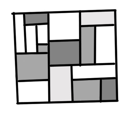
Now, after developing the basic parametric structure of Subscapes terrains, I started to build out the rendering and drawing components. A common trait in the output is subdividing the surface into recursively smaller rectangles, to give it a patchwork quilt look.
For this, I used a structure known as a quadtree. Start with a 2D rectangle, then subdivide it into two child rectangles. Then, for each new child rectangle that is formed, split it again into two partitions, and so on, recursively for each new child, until you reach some stopping condition.
Several features here are randomly affected, such as the placement of the split point, the minimum desired rectangle size, which axis to split the partition along, the maximum depth of splits, and so on.
After splitting is finished, each ‘leaf node’ in the quadtree (i.e. rectangles with no children) form the final cells that make up the patchwork quilt. Each cell is given different attributes, such as stroke color and density.
Poisson Disk Sampling
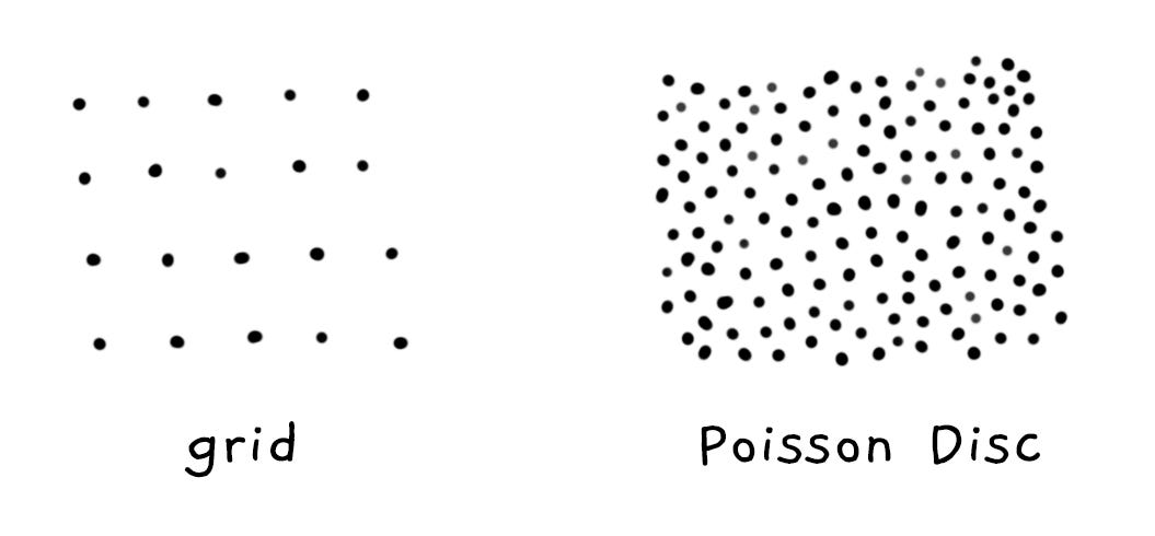
With parametric geometry, the surface is often split into horizontal and vertical slices, forming a uniform 2D grid. Drawing strokes at these grid points tends to produce a structured and mechanical result, but I wanted to achieve a more illustrative aesthetic. So, most Subscapes do not use a grid to place the stroke points, but instead create a distribution of Poisson Disk samples across the surface. This is a technique for creating points that are evenly spaced from each other, and often leads to a pattern that feels more natural.
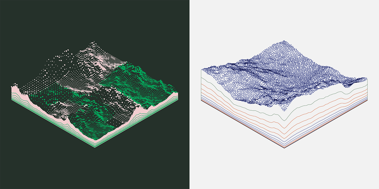
Notice how the stippled points are distributed on Subscapes #587 (using a grid for sampling) compared to #191 (using Poisson Disk distribution).
For reference, you can find a JavaScript implementation of Poisson Disk sampling in this notebook by Martin Roberts.
Flow Fields
The Grid-based or Poisson Disk sampling methods decide the starting point for each stroke across the surface, and then I use Flow Fields to create the organic motion of pen strokes tracing the contours of the terrain. Each stroke samples an (x, y) position from a noise function (different than the terrain noise) to determine a new angle of rotation, and from that we can offset the position by a vector pointing in this new direction.
See below for some pseudocode:
| // A 2D polyline of samples along a flow field | |
| let path = [ penStart ]; | |
| let [ x, y ] = penStart; | |
| for (let i = 0; i < steps; i++) { | |
| // Get new angle of rotation | |
| const angle = noise(x, y) * angleAmplitude; | |
| // Offset the point by this angle | |
| x += Math.cos(angle) * stepSize; | |
| y += Math.sin(angle) * stepSize; | |
| // Add the new sample | |
| path.push([ x, y ]); | |
| } |
Notice these samples are in 2D coordinates, not 3D. I use these as (u, v) coordinates into the parametric function, to determine the actual 3D coordinate of each vertex in the polyline stroke.
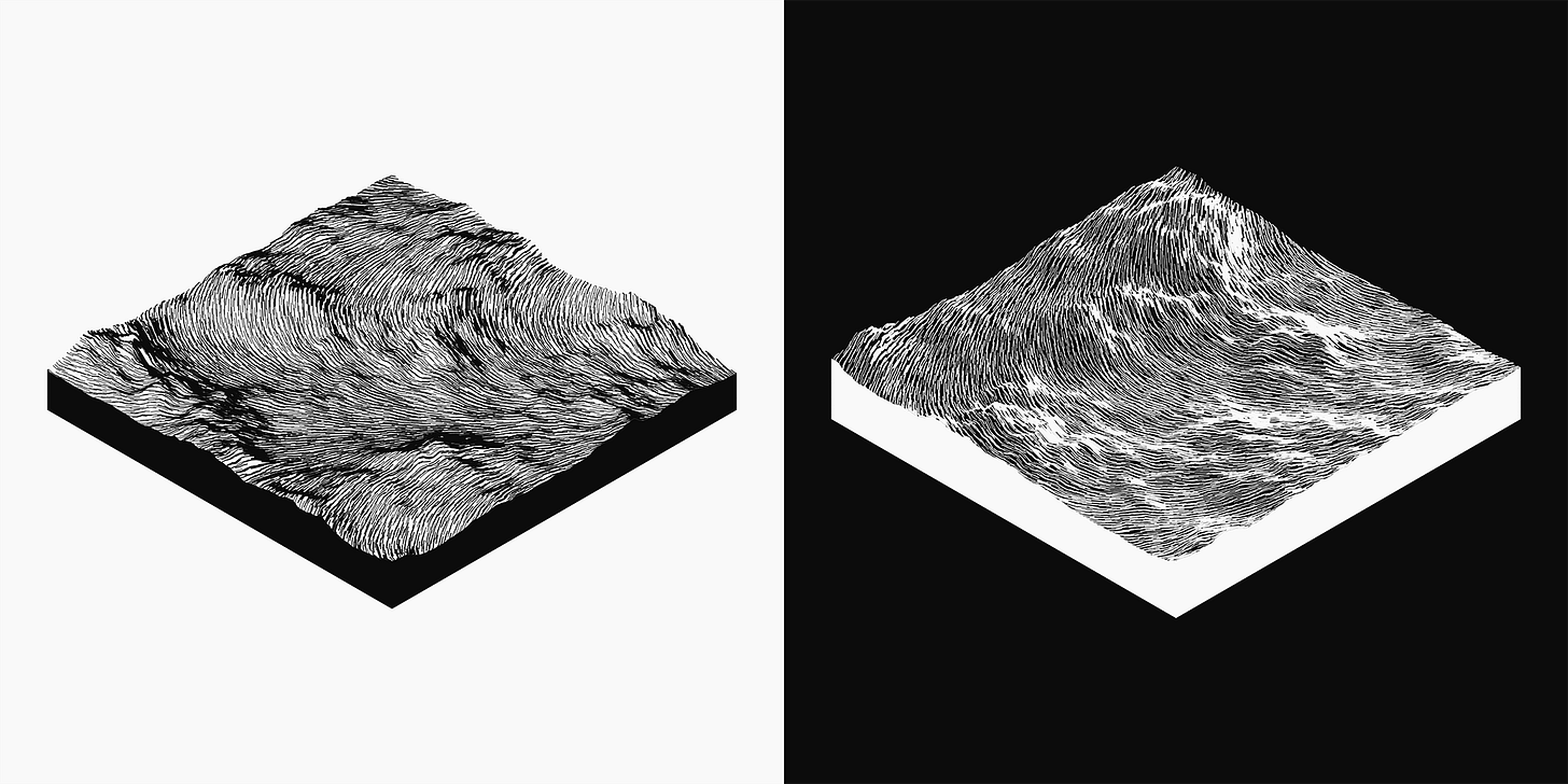
These undulating flow fields become more apparent on flat Subscapes, such as #270 and #623.
Flow fields can also be seen in various other ArtBlocks pieces, such as Tyler Hobbs’ Fidenza.
Raycasting
One drawback of using these 2D approaches for rendering 3D geometry is that the rendering has no concept of depth and occlusion: if you draw a complex mesh, all surfaces of it will be rendered, even if some surfaces in the mesh are occluded by other surfaces.
To fix this, I construct a high resolution triangle mesh from the parametric terrain. If a stroke vertex lies on a triangle that is facing away from the camera, it is culled. If the triangle faces the camera, I need to determine if any other triangles closer to the camera occlude it. This is done with raycasting: I cast a ray from the stroke vertex to the camera, and if the ray intersects any other triangles in the mesh along the way, there is a good chance it is obscured and should not be rendered.
This is a pretty brute-force approach—it’s computationally expensive and doesn’t always produce accurate results. I had to set the raycast resolution quite low to achieve fast render times, which causes some artifacts (see below), but the on-chain code and tools supports an additional argument that runs the algorithm with a higher resolution raycaster at the expense of render time.
Diffuse Lighting
Most of the techniques discussed so far help make up the structure of the 3D geometry (and its 2D screen-space representation), but we can also help visually define the mesh with lighting and shading techniques. This is implemented by selecting different colors and thicknesses for each pen stroke, sometimes giving the effect that the mountain is lit by a single light source from one side.
I use Lambertian Shading (sometimes called Diffuse Lighting) to determine the color intensity and thickness of each stroke. With our parametric function, we can assemble a geometric normal from 3 nearby samples, and then use “N dot L” (Lambert coefficient) to determine the diffuse contribution.
| const light = /* a unit normal for light direction */; | |
| // Determine the 3D position and normal from surface point | |
| const [ u, v ] = penStart; | |
| const [ position, normal ] = geometricNormal(parametricTerrain, u, v); | |
| // Get lambertian diffuse | |
| const diffuse = Math.max(0, vec3.dot(normal, light)); |
The color for each stroke is then interpolated through the current palette (such as dark to light colors) based on this diffuse intensity.
💡 Small detail: the algorithm reduces or “steps” the diffuse down to a discrete set of intensities, so instead of a value gradually changing between
0..1it may end up being one of[0, 0.3, 0.75, 1]or similar. The same is done for other features of the algorithm such as line thickness and sample density, as I found it produced a more illustrative output—in real life, you typically only have a small number of pen widths and colors to choose from!
The diffuse lighting technique is particularly visible in the Metallic styles, such as #229.
Procedural Color Selection
One challenge with Subscapes was color selection: not only was I constrained to a limited set of predefined colors (because the cost of uploading this data to the blockchain is expensive), but also the variety had to be such that it wouldn’t feel too repetitive over the course of 650 outputs. I decided to use a combination of predefined colors (many sourced from riso-colors and paper-colors), predefined palettes (some crafted by eye, others sourced from libraries like Kjetil Golid’s chromotome and Sanza Wada’s Dictionary of Colour Combinations), and procedurally random palettes.
The Screenprint and Lino traits are good examples of the procedural scheme, as I wanted a distribution of colors that were perceptually uniform in lightness, constrained in their chromaticity (i.e. saturation/colorfulness), and unbounded in their hue. For this, I used the OKLAB Color Space by Björn Ottosson, which is computationally cheap (and compact in byte size) and aims to be perceptually uniform. By sampling in cylindrical coordinates (LCh) it becomes easy to create a range of palettes for a particular aesthetic.
Here is some pseudocode that makes up both the Screenprint and Lino color palettes:
| import { LCh } from './color.js'; | |
| const isScreenprint = style === SCREENPRINT; | |
| const L = isScreenprint ? 50 : 92; | |
| const C = isScreenprint ? random.range(5, 20) : 5; | |
| const h = random.range(0, 360); | |
| const background = LCh(L, C, h); | |
| const foreground = isScreenprint ? 'white' : 'black'; |
Another common color task was to use a random predefined accent color, perhaps combined with a secondary color, and both of them overlaid atop a contrasting background color (in some cases the background is procedurally selected as above, in other cases the background is picked from a predefined set). To ensure all Subscape outputs meet a visual contrast criteria, I used an approach similar to what is defined in WCAG Color Contrast, using some parts of Tom MacWright’s wcag-contrast library.
There are lots of possible visually pleasing low-contrast palettes (such as the beautiful pixel artworks by @gijothehydroid), but in Subscapes I found that these palettes would look dull and washed out when compared next to higher contrast outputs.
Other Techniques
There’s many other ideas in the algorithm that I haven’t gone into, such as random gaussian distributions, shaping functions for different landscape types, constructing the tile base lines, and various bundling tools and source code optimizations. The above set of techniques are only a high level of the most significant parts of the algorithm.
Tokens as Data
Although I primarily wanted to break down the Subscapes rendering in this post, I also wanted to touch briefly on some of the other technical aspects of this project, and what makes it distinct from my past image and web-based generative artworks.
The Subscapes script is hosted within the data of an Ethereum smart contract; this means it is now ownerless and distributed and can no longer be changed by any single party, and it will persist in this immutable state for as long as the Ethereum blockchain continues to be validated and archived.
You can query the contract to verify this (for example, by reading GenArt721Core contract data from the blockchain with Etherscan). The immutability of the script is paired with the 650 unique tokens that were minted by ArtBlocks collectors during the artwork’s release, with each token being given its own unique hash that drives the artwork. This tokenization creates a novel form of digital ownership, secured by the blockchain and elliptic curve cryptography (public keys). Anybody can query the ownerOf() method in the same contract to determine which wallet currently holds which token. For example, token ID 53000000 identifies ArtBlocks Project 53 (Subscapes) and Token #0, which is currently assigned to my own public key (it is customary for ArtBlocks artists to mint and own the genesis token).
Many projects and applications are currently exploring some of the possibilities being enabled by this novel form of digital ownership; such as online galleries allowing collectors to showcase their digital walls (Showtime, Gallery.so, Oncyber, Artuego), as well as a growing interest in physical frames that display the owner’s held tokens, queried in real-time from the blockchain. Although this space is young, it is already allowing collectors to participate as curators, promoters, and investigators within specific styles and sub-fields of digital art. This is a distinct and positive shift away from previous roles of digital curation, such as an Instagram account that aggregates and highlights work from many artists, only to draw attention and revenue away from the artists and artworks they are featuring (eg. an Instagram aggregator publishing a highly compressed thumbnail image with no hyperlink to the work itself).
There are many APIs being built on top of this blockchain state (which acts as the single source of truth), such as Etherscan, OpenSea, Infura, and TheGraph, and browser wallets like Metamask provide a single-sign on flow for users to interact with decentralized web applications. To better understand these platforms myself, I have been building a few simple demos such as an online gallery, ArtBlocks renderer, and e-ink digital art frame.
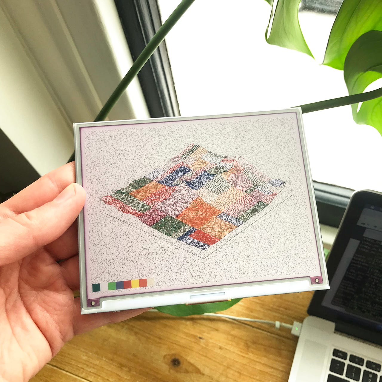
As an example; below is a simple code query for the ArtBlocks subgraph that fetches the ArtBlocks tokens currently held by the specified address. The same subgraph can be queried for project metadata, scripts, recent OpenSea trades, and other real-time data.
| { | |
| tokens(where: { owner: "... wallet address ..." }) { | |
| id | |
| project { | |
| name | |
| artistName | |
| } | |
| } | |
| } |
You can find a full JavaScript example of this here, which runs in Node.js and the browser.
Final Thoughts
It’s now been some months since the release of Subscapes on ArtBlocks.io, and the project has continued to grow and find new interest in the community. Several collectors have now received physical artist-signed prints of their tokens, and others are have been working with the open source Subscapes tools to produce their own mechanical plotter prints at home. Some makers are beginning to experiment with the output data for CNC milling, to build physical sculptures from the digital software.
It’s been exciting to watch the enthusiasm and community gather around Subscapes and other ArtBlocks projects, and rewarding as an artist to create a generative artwork that persists beyond the fleeting attention of social media Likes, Retweets, and Upvotes. The revenue and royalties from this project gives me the financial freedom to focus more fully on generative art and open source tooling, and the immutability and security of the data and tokens ensures the project will have a long lifespan, with many years of collection and consideration ahead.
Source Code & References
At the moment, the core Subscapes algorithm is not fully open source—this is to maintain my own artistic IP and avoid commercialization. However, some parts of the code have been published in github.com/mattdesl/subscapes, including the vector math, PRNG, and color utilities, as well as tools to generate new PNG and SVG outputs beyond the limited set of 650 mints. I have also published a template, tiny-artblocks, for others looking to build similarly compact projects for ArtBlocks.io. Further, all of the code and demos shown in this blog post via Gist and CodeSandbox is free to use under the MIT license.
